JL Lemma, a demo
Imports and Setup
Reading package lists... Done
Building dependency tree... Done
Reading state information... Done
cm-super is already the newest version (0.3.4-17).
dvipng is already the newest version (1.15-1.1).
texlive-latex-extra is already the newest version (2021.20220204-1).
texlive-latex-recommended is already the newest version (2021.20220204-1).
0 upgraded, 0 newly installed, 0 to remove and 35 not upgraded.To ensure reproducability, we will initiate a NumPy random number generator and set a random seed.
JL From Scratch
In this section, we will start with a toy dataset and verify the claim made by the JL lemma. First, we state the lemma again:
Let \(\displaystyle D\) be a dataset of \(\displaystyle n\) points in \(\displaystyle \mathbb{R}^{d}\). For any \(\displaystyle \epsilon \in ( 0,1)\) and \(\displaystyle k\geqslant \frac{8\log( n)}{\epsilon ^{2}}\), there exists a linear map \(\displaystyle f:\mathbb{R}^{d}\rightarrow \mathbb{R}^{k}\), such that for any \(\displaystyle x,y\in D\):
\[ \begin{equation*} 1-\epsilon \leqslant \frac{||f( x) -f( y) ||^{2}}{||x-y||^{2}} \leqslant 1+\epsilon \end{equation*} \]
We start with a function to generate a data matrix \(X\) of shape \(d \times n\). Here, each element is sampled from a uniform distribution. Note that the JL lemma is agnostic to the nature of the data. The claim holds for any set of \(n\) points in \(\mathbb{R}^{d}\).
First, we have a functiont to compute the pair-wise distances between all the \(n\) points in the dataset and store them in an arryay of shape \(n \times n\). The diagonals are zero since each entry measures the distance of a point from itself. We will add \(1\) to each diagonal entry. The reason for this will become clear soon.
Set a value for \(\epsilon\), the quantity that controls the extent of distortion that we are willing to tolerate. Using \(\epsilon\) and \(n\), compute the lower bound for \(k\) as given by the JL lemma.
We can now put down the function that generates a random matrix:
With the matrix in place, we can perform the transformation.
Next, we have a function that stores the distances between the original dataset and the transformed dataset.
The following function checks if the distortions are within the allowed limits for all the data-points in the dataset. It returns False if even a single pair of points suffer a distortion outside the given range. It returns True for a valid \(\epsilon\)-isometry.
All the functions we need are in place. Now, we go ahead and compute the \(\epsilon\)-isometry.
Code
Number of data-points = 5000
Dimension of parent space = 10000
Distortion limit, eps = 0.2
Dimension of projected space = 1704
Code
# Computing the eps-isometry
ratio_dist = np.array([2, ])
iter = 0
while not(is_eps_isometry(ratio_dist, eps)):
    M = get_matrix(k, d)
    X_t = transform(X, M)
    trans_dist = get_dist(X_t)
    ratio_dist = get_ratio(orig_dist, trans_dist)
    iter += 1

print(f'Approximate Isometry found after {iter} iterations!')
print(f'Maximum distortion = {ratio_dist.max()}')
print(f'Minimum distortion = {ratio_dist.min()}')
Approximate Isometry found after 2 iterations!
Maximum distortion = 1.1980556470711285
Minimum distortion = 0.823782054955422Effect of \(k\) on pair-wise distances
We will now turn to the effect of the projecting dimension on the pair-wise distances. To visualize this, we will look at the scatter of the pair-wise distances before and after the projection. On the side, we will also plot the histogram of the ratio of these distances.
Code
Number of data-points = 1000
Dimension of parent space = 2000
Distortion limit, eps = 0.1
Dimension of projected space = 5527
Code
# Run experiment for different values of k
for i, k in enumerate([100, 400, 1000]):
    M = get_matrix(k, d)
    X_t = transform(X, M)
    orig_dist = get_dist(X)
    trans_dist = get_dist(X_t)
    scale = max(orig_dist.max(), trans_dist.max())
    ratio_dist = get_ratio(orig_dist, trans_dist)

    # Scatter of original-transformed pair-wise distances
    plt.subplot(3, 2, 2*i + 1)
    x_ = np.linspace(0, 1, 2)
    plt.plot(x_, x_, alpha=0.9, linestyle='--', color='black')
    plt.axhline(linestyle='--', color='black',
                alpha=0.5)
    plt.axvline(linestyle='--', color='black',
                alpha=0.5)
    plt.scatter(orig_dist/scale, trans_dist/scale,
                alpha=0.05)
    plt.xlabel('Original distances')
    plt.ylabel('Transformed distances')
    plt.axis('equal')
    plt.title(f'k = {k}')

    # Histogram of distance ratios
    plt.subplot(3, 2, 2*i + 2)
    plt.hist(ratio_dist,
             bins=list(np.linspace(0, 2, 20)),
             edgecolor='black')
    plt.title('Histogram of ' + r'$\cfrac{d_{\text{trans}}}{d_{\text{orig}}}$')
    plt.tight_layout()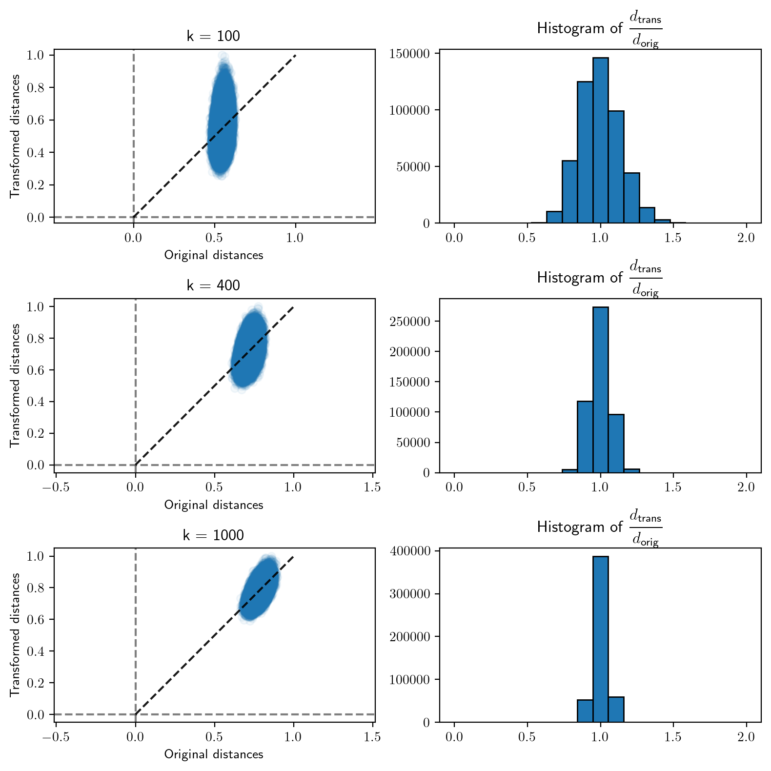
Visualizing random projections
We will now study the effect of multiplying a random matrix with a vector. To keep things simple, we will consider a \(2 \times 2\) matrix \(M\), all of whose entries are sampled from \(N(0, 1)\) and see what it does the unit vector \(e = (1, 0)\). This would require us to sample a number of random matrices and see where \(Me\) lands.
Code
# Distribution of Me
def plot_transforms():
    # plt.subplots(2, 2, constrained_layout=True)
    for i, m in enumerate([10, 100, 1_000, 10_000]):
        alpha = [0.5, 0.2, 0.1, 0.05]
        plt.subplot(2, 2, i + 1)
        th = np.linspace(0, 2*np.pi, 100)
        plt.plot(np.cos(th), np.sin(th),
                linestyle='--', color='black',
                alpha=0.5)
        plt.axhline(linestyle='--', color='black',
                    alpha=0.5)
        plt.axvline(linestyle='--', color='black',
                    alpha=0.5)
        plt.scatter([1], [0], color='red', alpha=1)

        proj, ang = mass_transform(m)
        plt.scatter(proj[0], proj[1], alpha=alpha[i])
        plt.xlim([-2, 2])
        plt.ylim([-2, 2])
        plt.title(f'{m} matrices')
    # plt.tight_layout()
plot_transforms()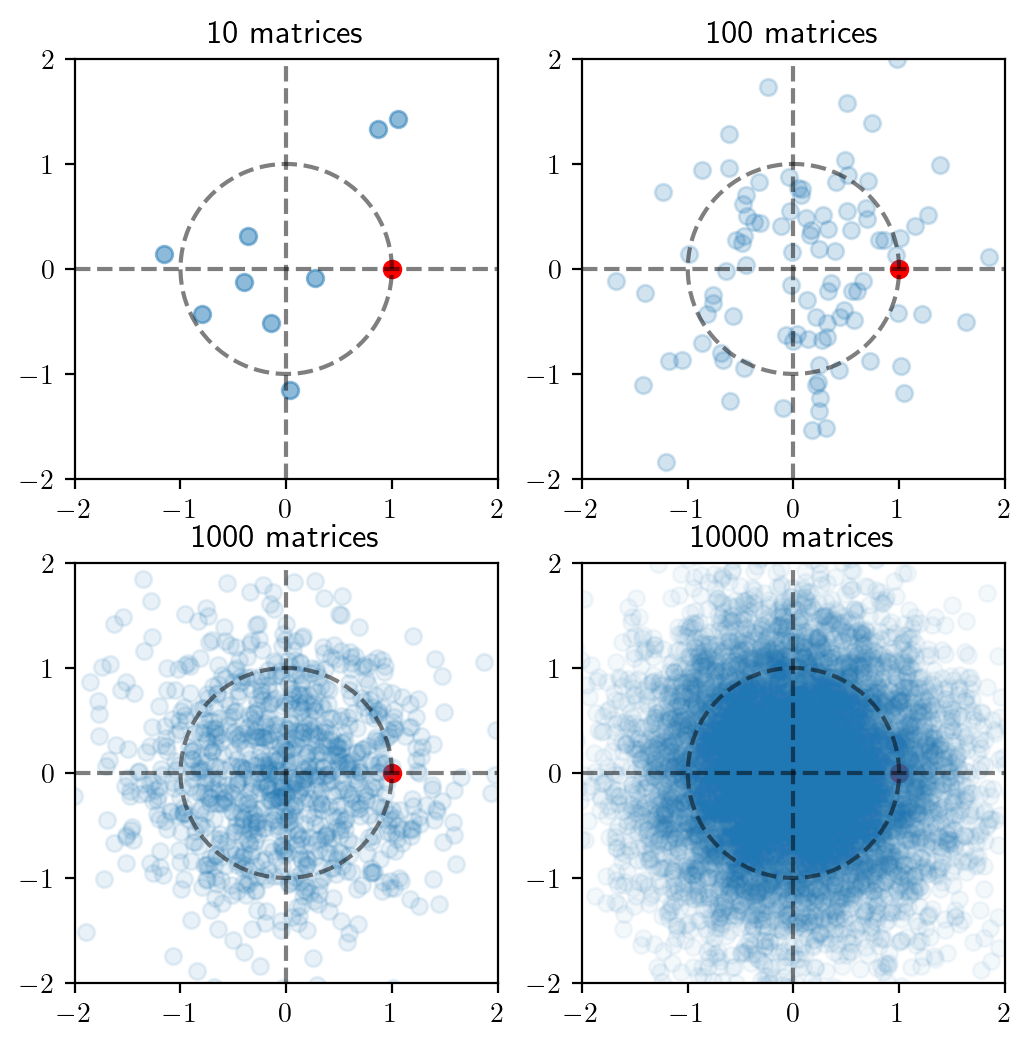
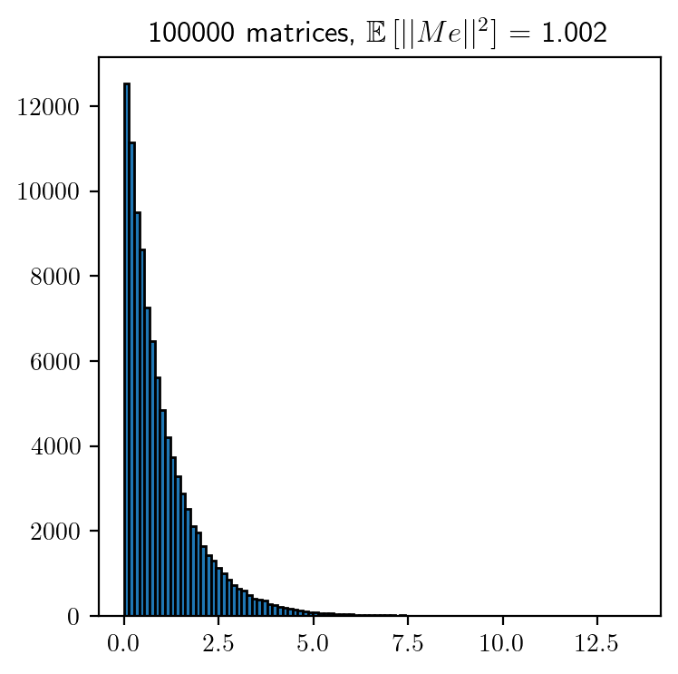
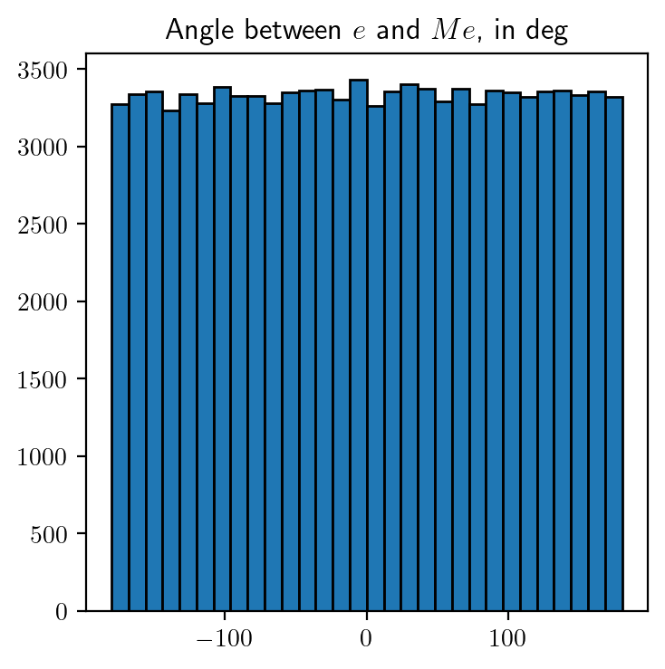
We will now study the distribution of \(||Me||^2\) by considering \(100,000\) random samples. Along with this, we will also study how the angle between \(e\) and \(Me\) is distributed.
Code
Interplay between \(\epsilon, n\) and \(k\)
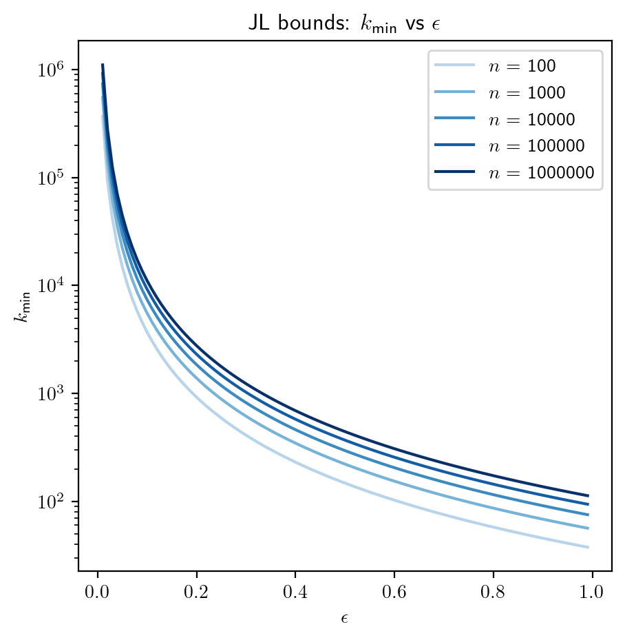
Recall that \(k \geqslant \cfrac{8 \log(n)}{\epsilon^2}\). We will use this bound to see how these three quantities impact each other.
Code
# Plot of k_min vs n
plt.rcParams['figure.figsize'] = [5, 5]

# range of admissible distortions
eps_range = np.linspace(0.1, 0.99, 5)
colors = plt.cm.Blues(np.linspace(0.3, 1.0, len(eps_range)))

# range of number of samples (observation) to embed
n_samples_range = np.logspace(1, 9, 9)

for eps, color in zip(eps_range, colors):
    k_min = 8 * np.log(n_samples_range) / (eps**2)
    plt.loglog(n_samples_range, k_min, color=color)

plt.legend([f"eps = {eps:0.1f}" for eps in eps_range], loc="lower right")
plt.xlabel(r"$n$")
plt.ylabel(r"$k_{\text{min}}$")
plt.title(r"JL bounds: $k_{\text{min}}$ vs $n$");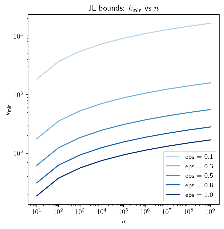
Code
# range of admissible distortions
eps_range = np.linspace(0.01, 0.99, 100)

# range of number of samples (observation) to embed
n_range = np.logspace(2, 6, 5)
colors = plt.cm.Blues(np.linspace(0.3, 1.0, len(n_range)))

plt.figure()
for n, color in zip(n_range, colors):
    k_min = 8 * np.log(n) / (eps_range**2)
    plt.semilogy(eps_range, k_min, color=color)

plt.legend([r'$n$' + f' = {int(n)}' for n in n_range], loc="upper right")
plt.xlabel(r"$\epsilon$")
plt.ylabel(r"$k_{\text{min}}$")
plt.title(r"JL bounds: $k_{\text{min}}$ vs $\epsilon$")
plt.show()